qrisp.gqsp.fourier_series_loader

fourier_series_loader(qarg: QuantumVariable, signal: ArrayLike | None = None, frequencies: ArrayLike | None = None, k: int = 1, mirror: bool = False) → QuantumBool

Performs quantum state preparation for the first \(k\) Fourier modes.

Given an input array of \(M\) values \(\{a_{j}\}_{j=0}^{M-1}\) representing a signal sampled at equidistant points, this method prepares an \(n\)-qubit quantum state \((N=2^{n})\) by reconstructing a smooth approximation of the signal using its lowest \(2k+1\) frequency components.

First, the method computes the frequency coefficients \(c_{l}\):

\[c_l = \frac{1}{M}\sum_{j=0}^{M-1} a_j e^{-i \frac{2\pi jl}{M}}\]

The method prepares the \(n\)-qubit state:

\[\ket{\psi} = \sum_{m=0}^{N-1} \psi_m \ket{m}\]

where the amplitudes \(\psi_{m}\) are computed using a band-limited inverse transform:

\[\psi_m = \frac{1}{\mathcal{K}}\sum_{l=-k}^k c_l e^{i \frac{2\pi lm}{N}}\]

In this expression, \(\mathcal{K}\) is a normalization constant ensuring \(\sum |\psi _{m}|^{2}=1\).

Parameters:

qargQuantumVariable

Variable representing the input signal. Must be in state \(\ket{0}\) for preparation of target signal.

signalArrayLike, shape (M,), optional

The target signal values. Either signal or frequencies must be specified.

frequenciesArrayLike, shape (2K+1), optional

The target frequency values in the range \([-K,K]\).

kint

The frequency cutoff. Only frequencies in the range \([-k,k]\) are preserved. The default is 1.

mirrorbool

If True, frequencies are caluclated from mirror padded signal via FFT to mitigate artifacts at the boundaries. The default is False.

Returns:

QuantumBool

Auxiliary variable after applying the GQSP protocol. Must be measured in state \(\ket{0}\) for the GQSP protocol to be successful.

Notes

• This method is particularly useful for preparing smooth states or approximating continuous functions where high-frequency noise should be filtered out.

• If (2k+1=M=N), this reduces to a standard state preparation from a full DFT.

Examples

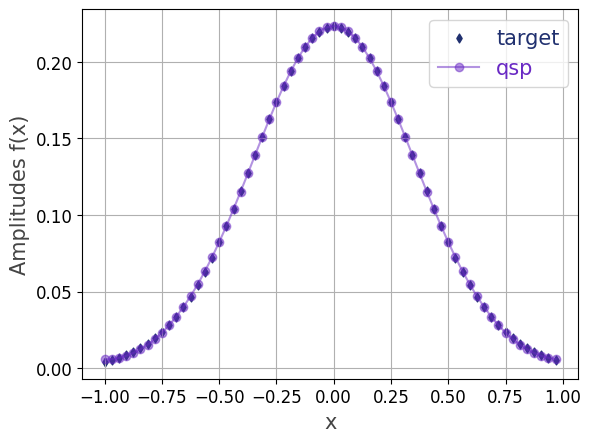
We prepare a quantum state with amplitudes following a Gaussian distribution.

# Restart the kernel to enable high-precision simulation
import os
os.environ["QRISP_SIMULATOR_FLOAT_THRESH"] = "1e-10"

import jax.numpy as jnp
import matplotlib.pyplot as plt
import numpy as np
from qrisp import *
from qrisp.gqsp import fourier_series_loader

# Gaussian
def f(x, alpha):
    return jnp.exp(-alpha * x ** 2)

# Converts the function to be executed within a
# repeat-until-success (RUS) procedure.
@RUS(static_argnames=["k"])
def prepare_gaussian(n, alpha, k):
    # Use 32 sampling points to evaluate f
    N_samples = 32
    x_val = jnp.arange(-1.0, 1.0, 2.0 / N_samples)
    y_val = f(x_val, alpha)
    y_val = y_val / jnp.linalg.norm(y_val)

    qv = QuantumFloat(n)
    anc = fourier_series_loader(qv, y_val, k=k)
    success_bool = measure(anc) == 0
    reset(anc)
    anc.delete()
    return success_bool, qv

# The terminal_sampling decorator performs a hybrid simulation,
# and afterwards samples from the resulting quantum state.
@terminal_sampling
def main(n, alpha):
    qv =  prepare_gaussian(n, alpha, 3)
    return qv

# Run the simulation for n-qubit state
n = 6
alpha = 4
res_dict = main(n, alpha)
y_val_sim = np.sqrt([res_dict.get(key, 0) for key in range(2 ** n)])

# Compare to target amplitudes
x_val = np.arange(-1, 1, 2 ** (-n + 1))
y_val = f(x_val, alpha)
y_val = y_val / np.linalg.norm(y_val)

plt.scatter(x_val, y_val, color='#20306f', marker="d", linestyle="solid", s=20, label="target")
plt.plot(x_val, y_val_sim, color='#6929C4', marker="o", linestyle="solid", alpha=0.5, label="qsp")
plt.xlabel("x", fontsize=15, color="#444444")
plt.ylabel("Amplitudes f(x)", fontsize=15, color="#444444")
plt.legend(fontsize=15, labelcolor='linecolor')
plt.tick_params(axis='both', labelsize=12)
plt.grid()
plt.show()

To perform quantum resource estimation, replace the @terminal_sampling decorator with @count_ops(meas_behavior="0"):

@count_ops(meas_behavior="0")
def main(n, alpha):
    qv =  prepare_gaussian(n, alpha, 3)
    return qv

main(6, 4)
# {'h': 6, 'rz': 8, 'p': 108, 'x': 6, 'cx': 72, 'rx': 7, 'measure': 1}