qrisp.QuantumSession.statevector

QuantumSession.statevector(return_type='sympy', plot=False, decimals=None)

Returns a representation of the statevector. Three options are available:

• sympy returns a Sympy quantum state, which is great for visualization and symbolic investigation. The tensor factors are in the order of the creation of the QuantumVariables (or equivalently: as they appear, when listed in print(self)).

• latex returns the latex code for the Sympy quantum state.

• function returns a statevector function, such that the amplitudes can be investigated by calling this function on a dictionary of this QuantumSession’s QuantumVariables.

If you need to retrieve the statevector as a numpy array, please use the corresponding QuantumCircuit method.

Parameters

return_typestr, optional

String indicating how the statevector should be returned. Available are sympy, array and function. The default is sympy.

plotbool, optional

If the return type is set to array, this boolean will trigger a plot of the statevector. The default is False.

decimalsint, optional

The decimals to round in the statevector. The default is 5 for return type sympy and infinite otherwise.

Returns

sympy.Expression or LaTeX string or function

An object representing the statevector.

Examples

We create some QuantumFloats and encode values in them:

>>> from qrisp import QuantumFloat
>>> qf_0 = QuantumFloat(3,-1)
>>> qf_1 = QuantumFloat(3,-1)
>>> qf_0[:] = 2
>>> qf_1[:] = {0.5 : 1, 3.5: -1j}

This encoded the state

\[\ket{\psi} = \ket{\text{qf_0}} \ket{\text{qf_1}} = \frac{1}{\sqrt{2}} \ket{2} (\ket{0.5} - i \ket{3.5})\]

Now we add qf_0 and qf_1:

>>> qf_res = qf_0 + qf_1

This gives us the state

\[\ket{\phi} = \frac{1}{\sqrt{2}}(\ket{2}\ket{0.5}\ket{2 + 0.5} - i \ket{2} \ket{3.5}\ket{2 + 3.5})\]

We retrieve the statevector as a Sympy expression:

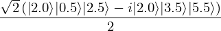
>>> sv = qf_0.qs.statevector()
>>> print(sv)
sqrt(2)*(|2.0>*|0.5>*|2.5> - I*|2.0>*|3.5>*|5.5>)/4

If you have Sympy’s pretty printing enabled in your IPython console, it will even give you a nice Latex rendering:

>>> sv

This feature also works with symbolic parameters:

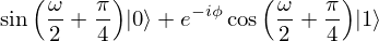
>>> from qrisp import QuantumVariable, ry, h, p
>>> from sympy import Symbol
>>> qv = QuantumVariable(1)
>>> ry(Symbol("omega"), qv)
>>> h(qv)
>>> p(-Symbol("phi"), qv)
>>> qv.qs.statevector()

Note

Statevector simulation with symbolic parameters is significantly more demanding than simulation with numeric parameters.

To retrieve the above expressions as latex code, we use return_type = "latex"

>>> print(qf_0.qs.statevector(return_type = "latex"))
'\frac{\sqrt{2} \left({\left|2.0\right\rangle }
{\left|0.5\right\rangle } {\left|2.5\right\rangle }
- i {\left|2.0\right\rangle } {\left|3.5\right\rangle }
{\left|5.5\right\rangle }\right)}{2}'

We can also retrieve the statevector as a Python function:

>>> sv_function = qf_0.qs.statevector("function")

Specify the label constellations:

>>> label_constellation_a = {qf_0 : 2, qf_1 : 0.5, qf_res : 2+0.5}
>>> label_constellation_b = {qf_0 : 2, qf_1 : 3.5, qf_res : 2+3.5}
>>> label_constellation_c = {qf_0 : 2, qf_1 : 3.5, qf_res : 4}

And evaluate the function:

>>> sv_function(label_constellation_a)
(0.7071048-1.3411045e-07j)

This is the expected amplitude up to floating point errors.

To get a quicker understanding, we can tell the statevector function to round the amplitudes using the round keyword.

>>> sv_function(label_constellation_b, round = 6)
(-0-0.707105j)

Finally, the last amplitude is 0 since the state of qf_res is not the sum of qf_0 and qf_1.

>>> sv_function(label_constellation_c, round = 6)
0j